You can fool people with math. It's quite easy. Here is my favourite trick (from Jaynes, 2003, p.452).
We define an infinite series $a_n$ ($n \gt 0$) along with its sum $S=\sum_i a_i$. The sum of the first $n$ terms is $s_n = \sum_{i=1}^n a_i$ and we also define $s_0=0$. It follows that $a_n=s_n-s_{n-1}$ Then a person in audience is asked to choose a number. Say, the person chooses $42$. We now claim that $S=42$ regardless of the definition of $a_n$ . Audience gasps with disbelief. Now the magic starts. It trivially follows that
$$a_n=s_n-s_{n-1}=s_n-42-s_{n-1}+42=(s_n-42)-(s_{n-1}-42)$$What is then $S$? $$S=(s_1-42)+(s_2-42)+(s_3-42)+ \dots$$ $$\ \ -(s_0-42)-(s_1-42)-(s_2-42)- \dots$$
The terms $(s_1-42),(s_2-42),(s_3-42),\dots$ cancel out. What remains is $S=-(s_0-42)=42$. Amazing!
Audience gasps with disbelief. An isolated nervous chuckle is heard from the back. Then the applause ensues. The croud cheers the magician. Either magic works or 42 is indeed the answer to everything! In any case it's an amazing result.
In statistics there is a reliable procedure for generating similarly amazing tricks (they are often called paradoxes). It works like this.
Algorithm $A_1$:
- Take two different models of the data-generating process $M_1$ and $M_2$.
- Hide the fact that these are two different models from the audience. This can be most elegantly done by a choice of two models that produce identical results in most cases but wildly diverge for few cases . Leaving out the details of the two models also helps.
- Select and demonstrate a case where the divergence is most visible. Since the two models are "identical" this should not happen. Ergo magic works!
An example of this procedure are "demonstrations" of nonconglomerability by Stone (1976; for brief description go here).
The magic generating Algorithm is also popular in the Frequentist vs Bayesian wars, where it usually adopts the following form.
Algorithm $A_2$:
- as in $A_1$.
- as in $A_1$.
- Select two procedures $P_F$ and $P_B$ for evaluating the models $M_1$ and $M_2$ respectively.
- Select and demonstrate a case where one of the models fails miserably. Pair the procedures with the models such that the disfavoured procedure is applied along with the faulty model. Since the two models are "identical" it is not the model but the procedure that fails. Ergo, this Procedure should be abandoned!
Rouder and colleagues push a new paper where they deconstruct frequentist confidence intervals. They work some serious stage magic along the lines of $A_2$.
Here is what they tell us. Consider the following example (p.3):
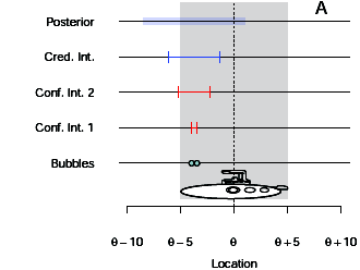
A 10-meter-long research submersible with several people on board has lost contact with its surface support vessel. The submersible has a rescue hatch exactly halfway along its length, to which the support vessel will drop a rescue line. Because the rescuers only get one rescue attempt, it is crucial that when the line is dropped to the craft in the deep water that the line be as close as possible to this hatch. The researchers on the support vessel do not know where the submersible is, but they do know that it forms distinctive bubbles. These bubbles could form anywhere along the craft’s length, independently, with equal probability, and float to the surface where they can be seen by the support vessel. The situation is shown in Figure 2A. The rescue hatch is the unknown location $\theta$, and the bubbles can rise anywhere from $\theta−5$ meters (the bow of the submersible) to $\theta$+5 meters (the stern of the submersible). The rescuers want to use these bubbles to learn where the hatch is located
Here is their Figure 2A:
The unconfident frequentist
The authors then claim that frequentist ($P_F$) assumes that the bubbles are generated by the normal distribution with unknown variance ($M_1$). The frequentist then computes the following confidence interval $\mathrm{CI}=m \pm t_{\alpha/2}s/\sqrt N$ where $m$ is the mean and $s$ is the standard deviation and N is the sample size. For two observations $x_1, x_2$ and $\alpha=0.5$ we get $m=(x_1+x_2)/2$ and $s=|x_1-x_2|/\sqrt{2}$ and
$$CI=m \pm \frac{|x_1-x_2|}{2}$$This result is shown in the figure in the second row from bottom. Following issues arise. When the two bubbles are near one another (left panel) the CI falsely claims high precision. In this situation, we can't say where the hatch is. The two bubbles could come from the bow or from the stern, but we don't know. When the two bubbles are far apart (right panel), one of them is at the bow and the other is at the stern. We then know with high precision that the hatch could be only located halfway between them. In this case instead CI incorrectly shows low precision.
The credible bayesian
Next, the authors demonstrate how bayesian ($P_B$) obtains plausible precision interval. Bayesian estimates
$$p(\theta|x) \propto p(x|\theta)p(\theta)$$Assume $p(\theta) \propto 1$. The observations are generated from the uniform distribution (not normal! hence $M_2$)
$$p(x|\theta)= \prod_i [x_i \lt \theta+5][x_i \gt \theta-5]/10$$($[\cdot ]$ is the Iverson Bracket)
As a result
$$p(\theta|x) \propto [\max(x_1,x_2)-5 \lt \theta][\min(x_1,x_2)+5 \gt \theta]$$The posterior of $\theta$ is unifom distribution with mean $m=(x_1+x_2)/2$ and range of $|x_1-x_2|-10$. Then the 50 % interval for $\theta$ (a.k.a. credible interval) is $m \pm (|x_1-x_2|-10)/2$. In the figure, the posterior is shown in the first row and the 50 % credible interval is in the second row. The width of credible interval corresponds to our intuitions.
Rouder et al. argue that confidence intervals should be discarded and we should use credible interval instead.
The incredible bayesian
Now here is how the show is performed at Café Fischer. A good Bayesian ($P_B$) really shouldn't choose uniform distribution as a prior as we did above. It is highly unlikely that the lost submersible has been carried 1000 miles away from point of initial submersion point $\theta_0$. Therefore a gaussian prior parametrized by mean $\theta_0$ and standard deviation $\sigma_0$ is a much better choice. Then we choose the likelihood to be a conjugate distribution to the prior as is common in bayesian inference. This means that $p(x|\theta)$ is gaussian ($M_1$), i.e. $x_i \sim \mathcal{N}(\theta,\sigma)$. Next, we add a scaled inverse $\chi$ prior for $\sigma$ and marginalize over it. The posterior is a student's $t$ distribution. Discarding the negligible influence of the prior we obtain a 50% credible interval for $\theta$ that is identical to the CI of the unconfident frequentist.
The confident frequentist
The stage is set for the confident frequentist ($P_F$) to save the crew in the submersible from drowning. He assumes uniform sampling distribution ($M_2$) and derives the corresponding likelihood function. $$\mathcal{L}(\theta; x_1,x_2)= \prod_i [x_i \lt \theta+5][x_i \gt \theta-5]/10$$ Next, he derives the ML estimate $\hat \theta = (x_1+x_2)/2$
We look up the definition of confidence interval in Wasserman (2004) in Section 6.3.2.:
A $1 − \alpha$ confidence interval for a parameter $\theta$ is an interval $C_n = (a, b)$ where $a = a(X1 , \dots , X_n )$ and $b = b(X1 , \dots , X_n )$ are functions of the data such that
$P_\theta(\theta \in C_n) \geq 1-\alpha $ for all $\theta \in \Theta$.
In our case the 50 % CI is obtained by solving for $y$ in
$$P_\theta(y>\theta - \hat \theta> -y)\geq 0.5$$where $\theta \sim \mathcal{U}(\max(x_1,x_2)-5,\min(x_1,x_2)+5)$.
This gives us the familiar CI $\hat \theta \pm y$ where $y= (|x_1-x_2|-10)/2$.
Conclusion
Above we saw all four procedures and method pairs in action $(P_F,M_1),(P_B,M_2),(P_F,M_2),(P_B,M_1)$. Clearly, whether a procedure fails depends exclusively on the model it assumes. In general, we should pay more attention to the choice of the appropriate model rather than the choice between bayesian and frequentist methods.
As for the statistician's stage magic, this can be useful tool for illustrating common confusions to students. The real danger then comes from people who managed to fool themself with their own stage tricks.