I will write lot about how statistical inference is done in psychological research. I think however that it will be helpfull to first point out few issues which I think are paramount to all my other opinions. In this post I write about the general attitude towards statistics that is imprinted on psychology students in their introductory stats classes.
Toolbox
This is how the statistics works for psychologists.
- Formulate hypothesis
- Design a study to test it
- Collect data
- Evaluate data
- Draw a conclusion and publish
When we zoom in at point 4 we get following instructions. First, see whether the data are at categorical, ordinal or nominal scale. Second, what design do we have? How many conditions/groups do we have? How many levels does each variable have? Do we have repeated measurements or independent samples? Once we have determined the answers we look at our toolbox and choose the appropriate method. This is what our toolbox looks like.
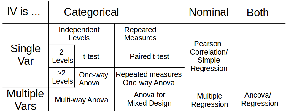
Then students are told how to perform the analyses in the cells with a statistical software, which values to copy from the software output and how one does report them. In almost all cases p-values are available in the output and are reported along with the test statistic. Since late 90s most software also offers effect size estimates and students are told where to look for them.
Let's go back to the toolbox table. As an example if we measured the performance of two groups (treatment group and control) at three consecutive time points then we have one nominal DV and two IVs: two independent groups and three repeated measurements. Looking at the table, we see that we have to perform Mixed-design Anova.
In the case where the scale of DV is not nominal the following alternative table is provided. Ordinal scale is assumed.
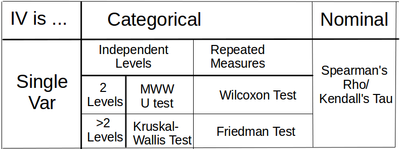
Finally, psychologists are also taught $\chi^2$ test which is applied when the DV is dichotomic categorical (i.e. count data).
That's the toolbox approach in a nutshell. It has problems.
Problems with toolbox
First, there is a discrepancy between how it is taught and how it is applied. The procedure sketched above is slavishly obeyed even when it doesn't make any sense. For instance, Anova is used as default model even in context where it is inappropriate (i.e. the assumptions of linearity, normality or heteroskedasticity are not satisfied).
Second, the above mentioned approach is intended as a one-way street. You can go only in one direction from step 1 to 5. This is extremely inflexible. The toolbox approach does not allow for the fitted model to be discarded. The model is fitted and the obtained estimates are reported. The 1972 APA manual captures the toolbox spirit: "Caution: Do not infer trends from data that fail by a small margin to meet the usual levels of significance. Such results are best interpreted as caused by chance and are best reported as such. Treat the result section like an income tax return. Take what's coming to you, but no more" One may protest that too much flexibility is a bad thing. Obviously, too much rigidity - reporting models that are (in hindsight but nevertheless) incorrect is not the solution.
Third, the toolbox implicitly claims to be exhaustive - it aplies as a tool to all research problems. Of course this doesn't happen and as a consequence two cases arise. First, inappropriate models are being fit and reported. We discussed this already in the previous paragraph. Second, the problem is defined in more general terms, such that not all available information (provided by data or prior knowledge) is used. That is, we throw away information so that some tool becomes available, because we would have no tool available if we included the information in the analysis. Good example are non-normal measurements (e.g. skewed response times) which are handled by rank tests listed in the second table. This is done even where it would be perfectly appropriate to fit a parametric model at the nominal scale. For instance we could fit response times with Gamma regression. Unfortunately, Gamma regression didn't make it into the toolbox. At other times structural information is discarded. In behavioral experiments we mostly obtain data with hierarchical structure. We have several subjects and many consecutive trials for each subject and condition. The across-trials variability (due to learning or order effects) can be difficult to analyze with the tools in the toolbox (i.e. time series methods are not in the toolbox). Common strategy is to build single score for each subject (e.g. average performance across trials) and then to analyze the obtained scores across subjects and conditions.
There is one notable strategy to ensure that you have the appropriate tool in the toolbox. If you can't fit a model to the data, then ensure that your data fit some tool in the toolbox. Psychologists devise experiments with manipulations that map the hypothesis onto few measured variables. Ideally the critical comparison is mapped onto single dimension and can be evaluated with a simple t-test. For example, we test two conditions which are identical except for a single manipulation. In this case we discard all the additional information and structure of the data since this is the same across the two conditions (and we do not expect that it will interact with the manipulation).
Unfortunately, there are other more important considerations which should influence the choice of design than the limits of our toolbox. Ecological validity is more important than convenient analysis. In fact, I think that this is the biggest trouble with the toolbox approach. It not only cripples the analysis, it also cripples the experiment design and in turn the choice of the research question.
Detective Work
Let's now have a look at the detective approach. The most vocal recent advocate has been Andrew Gelman (Shalizi & Gelman, 2013) but the idea goes back to George Box and John Tukey (1969). This approach has been most prevalent in fields that heavily rely on observational data - econometry, sociology and political science. Here, researchers were not able to off-load their problems to experimental design. Instead they had to tackle the problems head on by developing flexible data analysis methods.
While the toolbox approach is a one-way street, the detective approach contains a loop that iterates between model estimation and model checking. The purpose of the model checking part is to see whether the model describes the data appropriately. This can be done for instance by looking at the residuals and whether their distribution does not deviate from the distribution postulated by the model. Another option (the so-called predictive checking) is to generate data from the model and to look whether these are reasonably similar to the actual data. In any case, model checking is informal and doesn't even need to be quantitative. Whether a model is appropriate depends on the purpose of the analysis and which aspects of the data are crucial. Still, model checking is part of the results. It should be transparent and replicable. Even if it is informal there are instances which are rather formal up to the degree that can be written down as an algorithm (e.g. the Box-Jenkins method for analyzing time series). Once an appropriate model has been identified this model is used to estimate the quantities of interest. Often however the (structure of the) model itself is of theoretical interest.
An Application of Detective Approach
I already presented an example of detective approach when I discussed modeling of data with skewed distributions. Here, let's take a look at a non-psychological example which illustrates the logic of the detective approach more clearly. The example is taken from Montgomery, Jennings and Kulahci (2008). The data are available from the companion website.
%pylab inline
d= np.loadtxt('b5.dat')
t=np.arange(0,d.size)/12.+1992
plt.plot(t,d)
plt.gca().set_xticks(np.arange(0,d.size/12)+1992)
plt.xlabel('year')
plt.ylabel('product shipments');

The data are U.S. Beverage Manufacturer Product Shipments from 1992 to 2006 as provided by www.census.gov. The shipments show rising trend and yearly seasonal fluctuations. We first get rid of the trend to obtain a better look at the seasonal changes.
res=np.linalg.lstsq(np.concatenate(
    [np.atleast_2d(np.ones(d.size)),np.atleast_2d(t)]).T,d)
y=res[0][0]+res[0][1]*t
plt.plot(t, y)

plt.plot(t,d)
plt.gca().set_xticks(np.arange(0,d.size/12)+1992);

The fit of the linear curve is acceptable and we continue with model building. We now subtract the trend from the data to obtain the residuals. These show the remaining paterns in the data that require modeling.
plt.plot(t,d-y)
plt.gca().set_xticks(np.arange(0,d.size/12)+1992);
plt.ylim([-1000,1000]);
plt.ylabel('residuals')
plt.xlabel('year')

plt.figure()
plt.plot(np.mod(range(d.size),12)+1,d-y,'o')
plt.xlim([0.5,12.5])
plt.grid(False,axis='x')
plt.xticks(range(1,13))
plt.ylim([-1000,1000]);
plt.ylabel('residuals')
plt.xlabel('month');


We add the yearly fluctuations to the model. The rough idea is to use sinusoid $\alpha sin(2\pi (t+\phi))$ where $\alpha$ is the amplitude and $\phi$ is the shift. Here is a sketch what we are looking for. (The parameter values were found through trial and error).
plt.plot(np.mod(range(d.size),12)+1,d-y,'o')
plt.xlim([0.5,12.5])
plt.grid(False,axis='x')
plt.xticks(range(1,13))
plt.ylim([-1000,1000])
plt.ylabel('residuals')
plt.xlabel('month')
tt=np.arange(1,13,0.1)
plt.plot(tt,600*np.sin(2*np.pi*tt/12.+4.3));

We fit the model. We simplify the fitting process by writing $$\alpha sin(2\pi (t+\phi))= \alpha cos(2\pi \phi) sin(2\pi t)+\alpha cos(2\pi t) sin(2\pi \phi)= \beta_1 sin(2\pi t)+\beta_2 cos(2\pi t) $$
x=np.concatenate([np.atleast_2d(np.cos(2*np.pi*t)),
                np.atleast_2d(np.sin(2*np.pi*t))]).T
res=np.linalg.lstsq(x,d-y)
plt.plot(t,y+x.dot(res[0]))
plt.plot(t,d,'-')
plt.gca().set_xticks(np.arange(0,d.size/12)+1992);

The results look already good. We zoom in at the residuals, to see how it can be further improved.
ynew=y+x.dot(res[0])
from scipy import stats
plt.figure()
plt.hist(d-ynew,15,normed=True);
plt.xlabel('residuals')
print np.std(d-y)
r=range(-600,600)
plt.plot(r,stats.norm.pdf(r,0,np.std(d-ynew)))
plt.figure()
stats.probplot(d-ynew,dist='norm',plot=plt);


The residuals are well described by normal distribution with $\sigma=233$. We can summarize our model as $d=\beta_0+\beta_1 t + \beta_2sin 2\pi t + \beta_3sin 2\pi t + \epsilon$ with error $\epsilon \sim \mathcal{N}(0,\sigma)$
The plots below suggest some additional improvements.
plt.plot(t,d-ynew)
plt.ylabel('residuals')
plt.xlabel('year')
plt.gca().set_xticks(np.arange(0,d.size/12)+1992);

plt.figure()
plt.acorr(d-ynew,maxlags=90);
plt.xlabel('month lag')
plt.ylabel('autocorrelation');

plt.figure()
plt.plot(d,d-ynew,'o');
plt.ylabel('residuals')
plt.xlabel('predicted shipments');


The first two plots suggests a 9-year cycle. The third plot suggests that variance is increasing with time. Both suggestions are however difficult to evaluate because we don't have enough data.
Once we are satisfied with the obtained model we can look at the estimated parameter values if they conform to our predictions. The model can be also used to predict future shipments. For our purpose it was important to see the model building iteration and especially the model checking part. In this case model checking was done by inspecting the residuals. The presented case was rather straight-forward. If we tried to extend the model with a 9 year cycle or evolving variance this would require more thought and more detective work, which is the usual case with psychological data.
Better Results but More Work
Let's now evaluate detective approach by reviewing the problems caused by toolbox.
First, it seems difficult to make turn detective approach into ritual. Almost by definition it excludes this possibility. (Although I don't want to underestimate psychologist's ability to abuse any statistical method.)
Second, the approach is iterative. We are not required to stick to a model that we had in mind at the outset of our analysis.
Third, modeling is open-ended. The only limit is the computational tractability of the models, we would like to fit and the information afforded by the evidence.
Second and third point mean that detective approach is much more flexible and this flexibility can be abused. As stated above model building is an integral part of the reported results and all decisions should be made transparent, replicable accountable.
Finally detective approach requires more work. In particular, it requires the kind of work that researchers don't have time for - thinking. With toolbox you can get your students compute the p values. But he probably won't be able to accomplish the model building. This extra work is only a corollary of a general maxim that better results require more work. In future posts I will provide further illustrations that the better results afforded by detective approach are sorely needed.